I was one of those who discovered Bitcoin around 2012 and ignored it. I couldn’t find what its point was and I didn’t know “how much it costed”. Then, I was lucky to keep reading about it and jump into the Bitcoin train in 2013. A truly disrupting technology I wanted to be part of. Perhaps I invested more that I should have, but again, I was lucky and I got my investment back long time ago. Then Ethereum came in, then a ton of shitcoins. It’s a fun hobby from which I’m learning a lot.
For the last months I’ve been playing around with the financial aspect of the cryptocurrencies. A risky Forex I enjoy. It’s also helping me to improve my data science skills and analytic tools. Get data, clean it, summarize it, plot it. A kind of slow craft I feel proud of.
Thanks to that, I’ve seen the tight correlation among some pairs of cryptocurrencies. Most of the price displacement in one currency is almost instantly followed by a similar change in a different currency. This entanglement is mostly due to the arbitraging. For example, I have a position on the pair BTCUSD and I realize that the price goes suddenly up for whatever reason. If I’m fast enough, I can buy BTC in a different market where the price still down (let’s say selling ETH in ETHBTC), and sell the BTC from the cheap market (ETHBTC) on the expensive one (BTCUSD). Eventually the price for the same currency stabilizes itself across the different markets. The “eventually” part is a matter of seconds, not because I’m really fast, but because the trading is done by bots. These bots are constantly looking for arbitrage opportunities between pairs and even between exchanges. Difficult to beat the machine on many of the pairs, but what if there are some small pairs where bots are not that abundant and the stabilization of the price is slower?
For this post I’ll try to find correlations among the price of different cryptocurrencies paired with a stable currency such as the US Dollar.
Analysis
Libraries
First of all, I will load the libraries I will use during the script
library (data.table)    # Really eficient for large amount of data
library (ggplot2)       # Visualization
library (jsonlite)      # JSON retrieving
library (httr)          # API interaction
library (RcppRoll)      # Moving averages
Load data
To obtain the information for each pair, I will use CryptoWat.ch’s (CW) API. A very convenient, reliable, and free way to get almost every pair operated at the top crypto-exchanges.
I created a function retrieve the OHLC data from CW with only minutes and exchange as input.
ohlc.cw <- function (minutes, excha = "binance") {
    #Downloads the OHLC table from cryptowat.ch
    #
    # Arg:
    #   minutes: minutes from the moment the funcion is executed since
    #   the OHLC table will be taken
    #   excha: Any available exchange from CrytptoWat.ch
    #
    # Returns:
    #   A data.table with the Pair, Date, Price (in USDT) and
    #   6 Moving averages of 5, 10, 15, 20, 25, and 30 minutes span
    #

    # Use one method or the other depending of the OS
    if (Sys.info ()[[1]] == "Windows") {
        method_url = "wininet"
    } else {
        method_url = "curl"
    }

    # Time in unix format to pass to the API call
    after <- round ( (as.numeric (as.POSIXct (Sys.time ()))) - (minutes * 60), 0)

    # Get every pair of every exchange handle by Cryptowat.ch (JSON format)
    routes <- as.data.table (fromJSON ("https://api.cryptowat.ch/markets")$result)

    # Keep only info from Binance
    routes <- routes [grepl((excha), exchange),]

    # Drop non-active Pairs
    routes <- routes [active=="TRUE"]

    # Because I want only those currencies paired with USD, I will keep
    # the token USDT (ERC-20 token in parity with USD operated by Binance)
    routes <- routes [grepl(c("usdt"), pair),]

    # Create an empty data.table to hold data from the next loop
    all_pairs <- data.table ()

    # Loop to select the API route for each pair and obtain the OHLC for each one.
    for (i in 1: nrow (routes) ) {
        OHLC_json_exchange_pair <- as.data.table ((fromJSON (paste0 (routes$route[i], "/ohlc?periods=60&after=", after))$result$`60`))

        setnames (OHLC_json_exchange_pair,
                  c ("V1", "V2", "V3", "V4", "V5", "V6", "V7"),
                  c ("Time", "Open", "High", "Low", "Close", "VolumeToken", "VolumeBase"))

        fullTime <- data.table (Time = seq (from = range (OHLC_json_exchange_pair$Time)[1],
                                            to =  range (OHLC_json_exchange_pair$Time)[2],
                                            by = 60))

        OHLC_json_exchange_pair <- merge (OHLC_json_exchange_pair, fullTime,
                                          by = "Time", all = T)

        # I fill the ocassional NAs (no trades during that minute) given
        # by the API with the previous value
        for (j in 1:nrow (OHLC_json_exchange_pair)) {

            if (is.na (OHLC_json_exchange_pair$Open[j])) {

                OHLC_json_exchange_pair$Open[j] <- OHLC_json_exchange_pair$Open[j-1]
                OHLC_json_exchange_pair$High[j] <- OHLC_json_exchange_pair$High[j-1]
                OHLC_json_exchange_pair$Low[j] <- OHLC_json_exchange_pair$Low[j-1]
                OHLC_json_exchange_pair$Close[j] <- OHLC_json_exchange_pair$Close[j-1]
                OHLC_json_exchange_pair$VolumeToken[j] <- 0
                OHLC_json_exchange_pair$VolumeBase[j] <- 0

            }
        }

        # Add to the new table the pair
        OHLC_json_exchange_pair$Pair <- routes$pair[i]

        # Transform the unix time given by Binance to a more human-friendly date
        OHLC_json_exchange_pair$Date <- as.POSIXct (OHLC_json_exchange_pair$Time,
                                                    origin = "1970-01-01")

        # The final price is the average of the four (Open, High, Low, and Close)
        # values. `mean` is a slow command, btw.
        OHLC_json_exchange_pair [, price := (Open + High + Low + Close) / 4]

        # Moving averages for each pair
        OHLC_json_exchange_pair [, MA5 := roll_meanr (price, n = 5, na.rm = T)]
        OHLC_json_exchange_pair [, MA10 := roll_meanr (price, n = 10, na.rm = T)]
        OHLC_json_exchange_pair [, MA15 := roll_meanr (price, n = 15, na.rm = T)]
        OHLC_json_exchange_pair [, MA20 := roll_meanr (price, n = 20, na.rm = T)]
        OHLC_json_exchange_pair [, MA25 := roll_meanr (price, n = 25, na.rm = T)]
        OHLC_json_exchange_pair [, MA30 := roll_meanr (price, n = 30, na.rm = T)]

        # Remove some variables I'm not using
        OHLC_json_exchange_pair [, (1:7) := NULL]

        all_pairs <- rbind (all_pairs, OHLC_json_exchange_pair)
        rm (OHLC_json_exchange_pair)
    }

    return (all_pairs)
}
Using the above function, I create a data.table of the last 100 hours for every currency paired with the USD token.
OHLC <- ohlc.cw (60 * 100)Sanity check
head (OHLC, 30)## Pair Date price MA5 MA10 MA15
## 1: btcusdt 2018-07-23 07:27:00 7656.198 NA NA NA
## 2: btcusdt 2018-07-23 07:28:00 7659.245 NA NA NA
## 3: btcusdt 2018-07-23 07:29:00 7658.917 NA NA NA
## 4: btcusdt 2018-07-23 07:30:00 7659.010 NA NA NA
## 5: btcusdt 2018-07-23 07:31:00 7663.000 7659.274 NA NA
## 6: btcusdt 2018-07-23 07:32:00 7663.345 7660.704 NA NA
## 7: btcusdt 2018-07-23 07:33:00 7663.977 7661.650 NA NA
## 8: btcusdt 2018-07-23 07:34:00 7664.320 7662.730 NA NA
## 9: btcusdt 2018-07-23 07:35:00 7658.557 7662.640 NA NA
## 10: btcusdt 2018-07-23 07:36:00 7657.240 7661.488 7660.381 NA
## 11: btcusdt 2018-07-23 07:37:00 7655.927 7660.005 7660.354 NA
## 12: btcusdt 2018-07-23 07:38:00 7653.660 7657.941 7659.796 NA
## 13: btcusdt 2018-07-23 07:39:00 7652.700 7655.617 7659.174 NA
## 14: btcusdt 2018-07-23 07:40:00 7654.485 7654.802 7658.721 NA
## 15: btcusdt 2018-07-23 07:41:00 7656.920 7654.738 7658.113 7658.500
## 16: btcusdt 2018-07-23 07:42:00 7656.432 7654.840 7657.422 7658.516
## 17: btcusdt 2018-07-23 07:43:00 7654.405 7654.989 7656.465 7658.193
## 18: btcusdt 2018-07-23 07:44:00 7647.735 7653.995 7654.806 7657.448
## 19: btcusdt 2018-07-23 07:45:00 7645.195 7652.137 7653.470 7656.527
## 20: btcusdt 2018-07-23 07:46:00 7645.225 7649.798 7652.269 7655.342
## 21: btcusdt 2018-07-23 07:47:00 7651.648 7648.841 7651.841 7654.562
## 22: btcusdt 2018-07-23 07:48:00 7650.972 7648.155 7651.572 7653.695
## 23: btcusdt 2018-07-23 07:49:00 7650.398 7648.688 7651.342 7652.767
## 24: btcusdt 2018-07-23 07:50:00 7649.555 7649.560 7650.849 7652.167
## 25: btcusdt 2018-07-23 07:51:00 7651.505 7650.815 7650.307 7651.784
## 26: btcusdt 2018-07-23 07:52:00 7651.812 7650.849 7649.845 7651.510
## 27: btcusdt 2018-07-23 07:53:00 7651.123 7650.879 7649.517 7651.341
## 28: btcusdt 2018-07-23 07:54:00 7648.808 7650.561 7649.624 7651.081
## 29: btcusdt 2018-07-23 07:55:00 7648.730 7650.396 7649.977 7650.698
## 30: btcusdt 2018-07-23 07:56:00 7648.770 7649.849 7650.332 7650.154
## Pair Date price MA5 MA10 MA15
## MA20 MA25 MA30
## 1: NA NA NA
## 2: NA NA NA
## 3: NA NA NA
## 4: NA NA NA
## 5: NA NA NA
## 6: NA NA NA
## 7: NA NA NA
## 8: NA NA NA
## 9: NA NA NA
## 10: NA NA NA
## 11: NA NA NA
## 12: NA NA NA
## 13: NA NA NA
## 14: NA NA NA
## 15: NA NA NA
## 16: NA NA NA
## 17: NA NA NA
## 18: NA NA NA
## 19: NA NA NA
## 20: 7656.325 NA NA
## 21: 7656.097 NA NA
## 22: 7655.684 NA NA
## 23: 7655.258 NA NA
## 24: 7654.785 NA NA
## 25: 7654.210 7655.223 NA
## 26: 7653.634 7655.047 NA
## 27: 7652.991 7654.723 NA
## 28: 7652.215 7654.318 NA
## 29: 7651.724 7653.907 NA
## 30: 7651.300 7653.338 7654.327
## MA20 MA25 MA30Plotting all the things
To take a look to the correlation for each pair, I created a function with two different tokens as input and a metric (price or some MA). The metric for both currencies are normalized (mean divided by the standard deviation) so they can be compared easily on the same graph.
plot.metric <- function (tokenA_input, tokenB_input = "btc",  metric = "MA5") {
    # Creates plot showing a metric (i.e. "price") over time for two currencies
    #
    # Arg:
    #   tokenA_input: Token in three letters format
    #   tokenB_input: Token in three letters format
    #   metric: A metric to show from "price", "MA5", "MA10", "MA15", "MA20",
    #   "MA25", and "MA30".
    #
    # Returns:
    #     A plot with the selected metric for both currencies
    #

    tokenA <- paste0 (tokenA_input, "usdt")
    tokenB <- paste0 (tokenB_input, "usdt")

    # Reduce the size of the table to the values of the selected currencies
    dtPlot <- OHLC [Pair %in% c(tokenB, tokenA)]

    # Due to the disparity of the prices for each currency, I normalize the values
    # so they can be easily compared to each other
    dtPlot [, normalizedPrice := (get(metric) - mean (get (metric), na.rm = T))
            / sd (get(metric), na.rm = T), by = Pair ]

    ggplot (data = dtPlot, aes (x = Date)) +
        theme_classic () +

        theme (legend.position = "bottom") +

        geom_line (aes (y = normalizedPrice, color = Pair)) +
        labs (title = paste0 ("Normalization of the price (USDT) of ",
                              tokenA_input, " and ", tokenB_input),
              y = "") +
        scale_colour_brewer (palette = "Set1")
}
Just to know the available tokens, another function to list them.
list_tokens <- function (data = OHLC) {

    pairList <- unique (data$Pair)
    tokenList <- gsub ("usdt", "", pairList)
    return (tokenList)
}

list_tokens ()
## [1] "btc" "eth" "bcc" "neo" "ltc" "ada" "xrp" "tusd" "trx" "etc"
## [11] "qtum" "eos" "xlm" "ont" "icx" "bnb" "ven" "iot" "nuls"Using the function to create the graph plot.metric and choosing two currencies from the list and one metric
plot.metric ("eth", "btc", "MA30")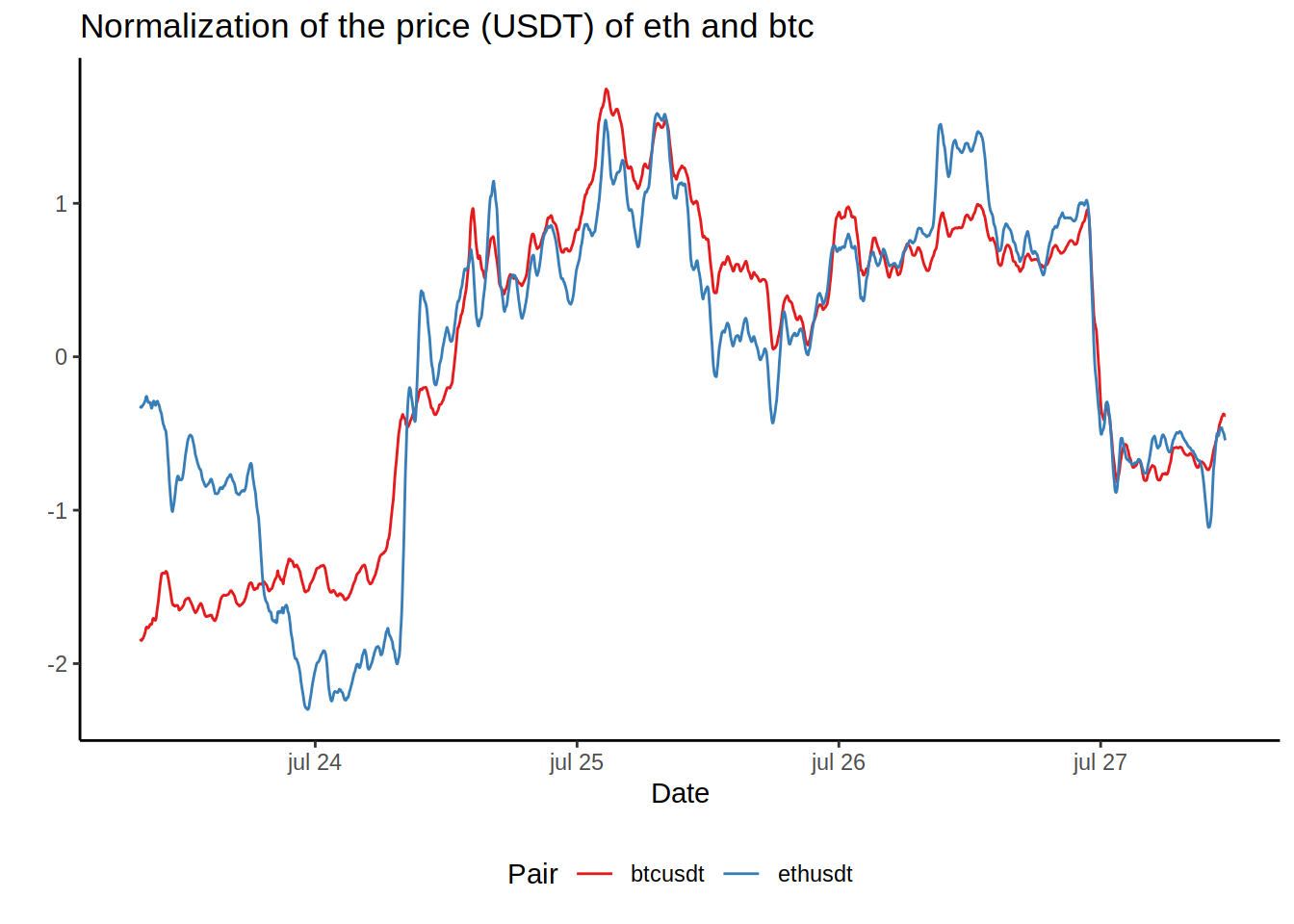
Correlation time
As the final step (for now), I’m creating a function to correlate the selected metric of every currency with a X-minutes delayed version of the same metric.
The function will show a table with the most extreme correlations (both negative and positive) and a heat map to visualise it more easily.
corr.delayed <- function (OHLC_table, delay, metric = "price") {
    # Correlate the metric of every token with the same delayed metric
    #
    # Arg:
    #   OHLC_table: OHLC table with info from different pairs
    #   delay: Delay (in minutes) to apply to the metric
    #   metric: A metric to show from "price", "MA5", "MA10", "MA15", "MA20",
    #   "MA25", and "MA30"
    #
    # Returns:
    #   The most extreme correlations of the metric and the delayed metric
    #   among all the pairs
    #   A heat map with the values of every correlation

    # Data.table creates copies by reference if the command `copy` is not used.
    OHLC_table <- copy (OHLC_table)

    # Create delayed variables from the metric and delay selected.
    for (d in 3:ncol (OHLC_table)) {
        colName <- colnames (OHLC_table)[d]
        OHLC_table [, paste0 (colName, "_delay_", delay) :=
                        shift (get (colName), n = delay, type = "lag"), by = Pair]
    }

    fusedData <- data.table (Date = OHLC_table$Date)

    # Loop to go through all the pairs and create a new table where the columns are the
    # value of the metric for each independent pair
    for (e in unique (OHLC_table$Pair)) {
        tmp <- OHLC_table [OHLC_table$Pair == e][,!1]

        colnames (tmp)[2:ncol(tmp)] <- paste0 (e, "_", colnames (tmp)[2:ncol(tmp)] )

        fusedData <- merge (fusedData, tmp, all.x = T)
    }

    # Selecting only the metric to be analyzed/plotted
    reducedFusedData <- fusedData [, grepl (metric, colnames (fusedData)), with = F]

    # The two variables to be analyzed for correlations
    # (the metric and the delayed metric)
    corX <- reducedFusedData [, !grepl ("delay", colnames (reducedFusedData)), with = F]
    corY <- reducedFusedData [,  grepl ("delay", colnames (reducedFusedData)), with = F]

    # Data.table with the correlation of the metrics
    # (only when both metrics are presents,
    # it'll drop some rows due the MA and the delayed values be filled with NAs)
    corplotDT <- as.data.table (melt (cor (x = corX, y = corY, use = "pairwise.complete.obs")))

    # Create heat map
     corplot <- ggplot (data = corplotDT, aes (x = Var1, y = Var2, fill = value)) +
        geom_tile () +

        theme(axis.text.x = element_text(angle = 45, hjust = 1),
              legend.position = "bottom") +
        guides (fill = guide_colorbar (barwidth = 10)) +

        labs (title = paste0 (metric, " vs. ", metric, " ", delay, "-minutes delay"),
              subtitle = "Correlation among cryptocurrencies",
              x = metric,
              y = paste ("Delayed", metric, "by", delay, "min", sep = " ")) +
        scale_fill_distiller (direction = 1, palette = "PiYG") # If you are **not** colorblind, change the palette to "RdYlGn"
    print (corplot)

    # Show a table with the autocorrelations removed ...
    orderedMeltedCorplot <- corplotDT [value != "1"][value != "-1", ]

    # ... correlations between the same pair also removed ...
    orderedMeltedCorplot <- orderedMeltedCorplot [orderedMeltedCorplot [, substr (Var1, 1, 7) != substr (Var2, 1, 7)]][order (-value)]

    # ... and the most correlated (both negatively and positively)
    orderedCor <- rbind (head (orderedMeltedCorplot, 3), tail (orderedMeltedCorplot, 3))
    return (orderedCor)
}
So let’s use it!
corrTable <- corr.delayed (OHLC_table = OHLC, delay = 10, metric = "price")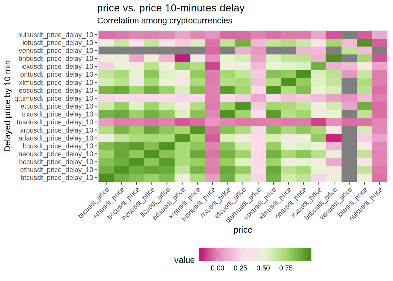
corrTable## Var1 Var2 value
## 1: bccusdt_price ltcusdt_price_delay_10 0.9613941
## 2: ltcusdt_price bccusdt_price_delay_10 0.9605355
## 3: eosusdt_price trxusdt_price_delay_10 0.9581390
## 4: icxusdt_price tusdusdt_price_delay_10 -0.1244779
## 5: bnbusdt_price adausdt_price_delay_10 -0.1621247
## 6: adausdt_price bnbusdt_price_delay_10 -0.1700144To keep the process automatic, I’m creating another function (yes, another one) to extract and plot the pairs with the highest (positive and negative) values of correlation.
top.corr.plot <- function (corrTable, topORbottom = "top") {
    # Correlate the metric of every token with the same delayed metric
    #
    # Arg:
    #   corrTable: Correlation table created with the function `corr.delayed`
    #   topORbottom: Choose between "top" for the most positvely correlated pairs
    #   or "bottom" for the most negatively correlated pairs.
    #
    # Returns:
    #  A line plot with the normalized prices in USDT for both pairs.

    if (topORbottom == "top") {
        tokenA <- gsub ("usdt_.*$", "", corrTable$Var1 [1])
        tokenB <- gsub ("usdt_.*$", "", corrTable$Var2 [1])
    } else {
        tokenA <- gsub ("usdt_.*$", "", corrTable$Var1 [6])
        tokenB <- gsub ("usdt_.*$", "", corrTable$Var2 [6])
    }
    plot <- plot.metric (tokenA = tokenA, tokenB = tokenB, metric = "price")
    print (plot)
}
So to create the plot for the most positively correlated tokens:
top.corr.plot (corrTable, topORbottom = "top")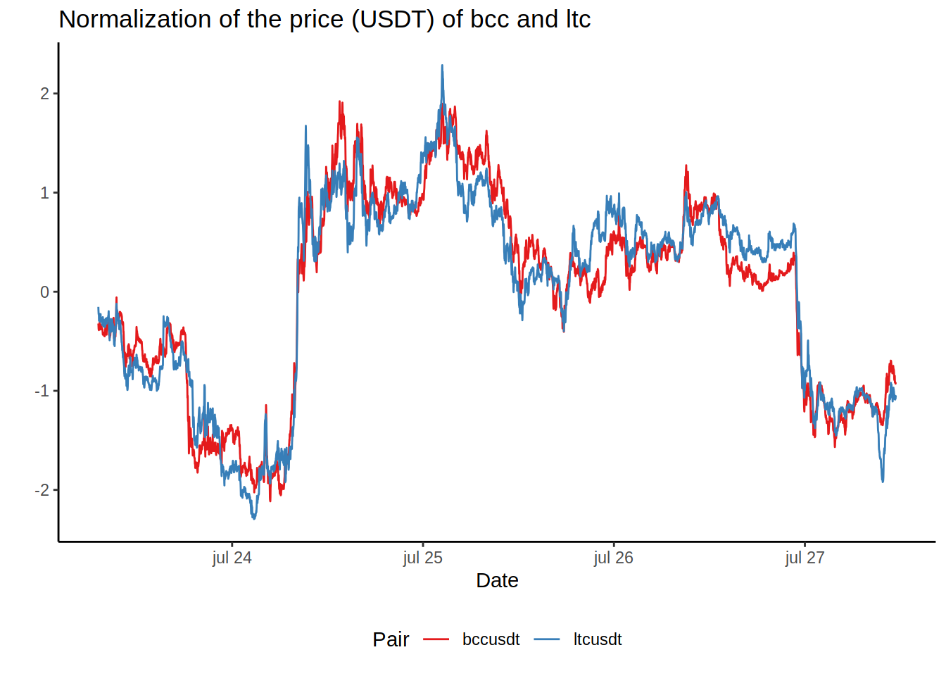
And conversely to create the plot for the most negatively correlated tokens:
top.corr.plot (corrTable, topORbottom = "bottom")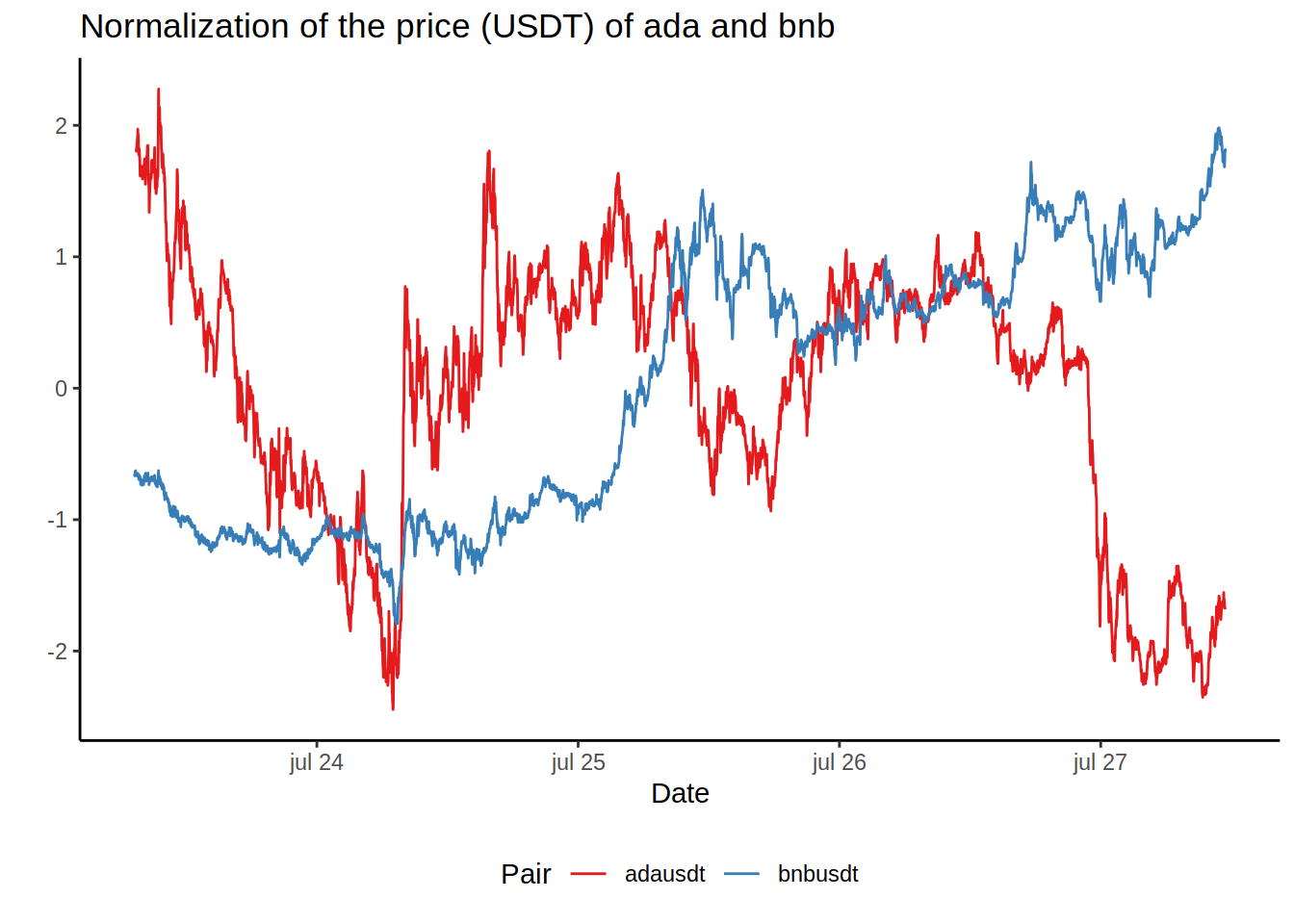
Conclusion
I’m not the first one to try to correlate currency markets. When the millionaire profits depend on milliseconds, the money at stake goes to any small advantage to be the smartest and the fastest. Here, I’ve playing around with numbers. Am I right about the correlations? Apparently during the period under study, yes, there are some insightful correlations. However, correlations do not mean causation and it does not mean that the same correlation will be the same after a period of time. Take this analysis with a ton of salt and don’t take it as a financial advise. Do your own research, please.
Also, this script is automatic and it depends on the API behaving. Review the graphs and tables looking for incongruences.
Next
I was going to do some machine learning predictions in this post, but it grew too much to do it now, but rest assured I will do it.
Next post, I will use some simple machine learning algorithms to try to predict the price of one currency based on the metric of other/s.